LIGO signal processing in two lines of code

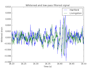
Two lines of signal processing will dig out the gravitational wave signal!

This year’s Nobel prize in physics was awarded to Rainer Weiss, Barry C. Barish, and Kip Thorn
for the discovery of gravitational waves. Only two years earlier, on September 14 2015, 09:50:45
UTC, the two Laser Interferometer Gravitational-Wave Observatory (LIGO) instruments detected
a gravitational wave for the first time in history. This event was perhaps the most important
scientific discovery since the detection of the Higg’s boson by CERN. The existence of gravitational
waves had been predicted by Einstein’s general theory relativity, but never before detected.

The gravitational wave event detected by LIGO is thought to be from a collision of two black
holes, which sends out a localized chirp like pulse in the space-time. LIGO utilizes two detectors,
which are spaced approximately 3000 km apart. These detectors measure strain (∆L/L) as a function of time. Here ∆L is the variation in length and L is the total length in which the variation is measured.
In other words, strain is the normalized variation in length L of the interferometer line due to
gravitational-wave induced ripples in space-time.

LIGO uses two geographically separated stations to measure gravitional waves: Hanford, WA
(H1), and Livingston, LA (L1). The gravitational wave propagates at the speed of light c ≈ 3e8
m/s. If the same signal is detected at two different places with a time difference less than or equal
to the speed of light propagation time between the sensors, then this provides assurance that the
event is in fact real, and not caused by e.g., local seismic activity. Now with three stations, triangulation can be used to determine direction of arrival for LIGO events!

The LIGO data is severely corrupted with instrumental noise. This noise is much larger in
amplitude than the gravitational wave signal. However, this noise is very narrow band in nature,
and it can be filtered out using relatively basic signal processing techniques. Such filtering is
routinely used by LIGO to improve the sensitivity of the instrument.

In fact the signal processing techniques are so simple that an undergraduate can implement them from scratch in a few weeks. That is exactly what I had my students do for their midterm exam in the signal processing course this year. Out of 46 students 45 managed to dig out the gravitational wave signal on their own, albeit with some specific instructions on what sort of techniques to use.

I didn't want the students to just copy the publicly available LIGO signal processing tutorial, so I though I'd send the students down a slightly different path, which is even more simple than the one in the tutorial. My course is a very basic one, which doesn't cover statistical aspects of signals, so this technique involves no statistical processing!

In fact, it is possible to boil down LIGO signal processing into just two lines of code. Here's what I came up with:

# Dig out the LIGO signal
# whiten spectrum and lowpass
def whiten_and_lp(z,L=8):
    Z=rfft(s.tukey(z.size)*z,z.size)
    return(irfft(rfft(n.repeat(1.0/L,L),z.size)*Z/n.abs(Z)).real)

Technically, I guess I could have reduced this to one line, but that wouldn't have fit the line width on this blog post.

The full code, which includes reading LIGO files and plotting is shown below. You can download the data here and here.

#!/usr/bin/env python
#
# Signal processing to clean up mechanical vibrations from LIGO data.
# The idea is to use very simple signal processing concepts. 
#
# (c) 2017 Juha Vierinen
#
import numpy as n
from numpy.fft import rfft
from numpy.fft import irfft
import h5py as h
import scipy.signal as s
import matplotlib.pyplot as plt

# Dig out the LIGO signal
# whiten spectrum and lowpass
def whiten_and_lp(z,L=8):
    Z=rfft(s.tukey(z.size)*z,z.size)
    return(irfft(rfft(n.repeat(1.0/L,L),z.size)*Z/n.abs(Z)).real)

# Read strain data
sh1=h.File("H-H1_LOSC_4_V2-1126259446-32.hdf5","r")["strain/Strain"].value
sl1=h.File("L-L1_LOSC_4_V2-1126259446-32.hdf5","r")["strain/Strain"].value

# sample rate (Hz)
fs=4096.0

# time vector (seconds)
t=n.arange(len(sh1))/fs

# Whiten and lowpass filter Livingston and Hanford signals
wsh1=whiten_and_lp(sh1)
wsl1=whiten_and_lp(sl1)

# Plot whitened and low-pass filtered signal
plt.plot(t,wsh1,label="Hanford")    
plt.plot(t,wsl1,label="Livingston") 
plt.xlabel("Time (s)")
plt.ylabel("Whitened strain")
plt.title("Whitened and low-pass filtered signal")
plt.legend()
plt.xlim([16.2,16.5])
plt.show()